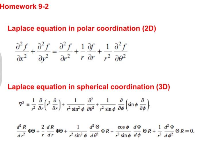
Lecture 7.4: The Laplacian In Polar Coordinates
Di: Ava
The p{Laplacian operator pu = div jrujp 2ru is not uniformly ellip-tic for any p 2 (1; 2) [ (2; 1) and degenerates even more when p ! 1 or p ! 1. In those two cases the Dirichlet and eigenvalue problems associated with the p-Laplacian lead to intriguing geometric questions, because their limits for p ! 1 or p ! 1 can be characterized by the geometry of . In this little survey I recall some Professor Berthold Horn, Ryan Sander, Tadayuki Yoshitake Department of Electrical Engineering and Computer Science Massachusetts Institute of Technology
7.1 Poisson and Laplace Equations The expression derived previously is the “integral form“ of Gauss’ Law Gregory Seregin – Lecture Notes on Regularity Theory for the Navier-Stokes Equations-World Scientific Publishing Co (2014) – Free download as PDF File (.pdf), Text File (.txt) or read online for free.
Class InformationProfessor Information The Laplacian and Some Natural Variants Our focus in this chapter is largely on the p-Laplacian. The theory of Chap. 1 con-cerning the representation of compact linear maps is used to establish the existence of a countable family of certain types of weak solutions of the Dirichlet eigenvalue problem for the p-Laplacian, with associated eigenvalues. This chapter gives a brief introduction to the spectral theory of graphs. The primary focus is on quantum graphs consisting of the Laplacian operator acting on a metric graph.
//Hyperion.maths.bris.ac.uk/macpd/ugt/apde2/notes/apde2.dvi
Integrating the strain-displacement relations provides the displacement field in terms of the bending moment and other parameters. The document also The techniques in [BDG] were extended by Simoes [SP] to show that even when pq, UP,q and VP,q passess homothety-invariant foliations by smooth minimizing hypersurfaces having CP,q as asymptote, provided p+q>5 and pq>5. Hardt and Simon [HS], subsequently observed that any area-minimiz- ing hypercone C which is smooth near infinity gives rise to this type of foliation. Spring 2019 lecture notes 18.04 Complex analysis with applications
The p{Laplacian operator pu = div jrujp 2ru is not uniformly ellip-tic for any p 2 (1; 2) [ (2; 1) and degenerates even more when p ! 1 or p ! 1. In those two cases the Dirichlet and eigenvalue problems associated with the p-Laplacian lead to intriguing geometric questions, because their limits for p ! 1 or p ! 1 can be characterized by the geometry of . In this little survey I recall some
The polar coordinates example above was presented in the context of Picture B. Picture B is the right picture for studying curvilinear coordinates where for example x-space = Cartesian coordinates and x‘-space = toroidal coordinates.
- Analysis on Manifolds via the Laplacian
- PartialDifferentialEquatio
- 6.801 / 6.866 Machine Version, Lecture Notes
with radius r. Temporarily take spherical polar coordinates centered at x. Average over the angles with respect to the angular measure sin d d =(4 ). An integration by parts shows that the contribution from the angular part of the Laplacian is zero.
{Hint: make use of polar coordinates x = r cos θ, y r sin and of the = θ expres-sion for the Laplacian in polar coordinates, r− 1( 1 = ∂r(r ∂r) (r− + ∂θ ∂θ )) . Observe that for such f the potential u does not depend on θ, and perform an analysis similar to that given above for the simplest differential equation of second order LECTURE 4-1 – Free download as PDF File (.pdf), Text File (.txt) or read online for free. The document provides an overview of quantum mechanics, focusing on its mathematical formalism, including key concepts such as Hilbert spaces, linear vector spaces, and the independent formulations of quantum mechanics by Heisenberg and Schrödinger. It discusses the
e Laplacian 1g is the trace of the Hessian: 1gu = trg Hessgu ( ) = giju;ij. Compare the component expressions at the center point of a normal coordinate chart for M ( Laplacian is often reserved for the case M g is Riemannian (though sometimes ( , ) defined as the negative of our definition), and in the case M g is Lorentzian, ( , CLO 3 : Explain Formula for Radius of curvature in Cartesian coordinates and Parametric coordinates and Polar coordinates CLO 4 : Explain Formation of Partial Differential Equations by eliminating the arbitrary constant and arbitrary functions CLO 5 : Explain Simple properties of definite Integrals and Bernoulli‘s Formula and Integration by (2019-08-21) It is now clear that the lectures will be in English. As a consequence, the exam will be given in English as well. (2019-06-03) I will be teaching the course in the fall of 2019. The lecture will be in English if required by at least one student. If you plan on taking the course, and need the lectures to be in English, drop me a line.
- Spring 2019 lecture notes
- Integrated density of states for the Poisson point interactions on
- On Cheeger constants of hyperbolic surfaces
- TMA4305 Partial Differential Equations 2019
- Fisher information for solutions of theBoltzmann equation
5.7 Solutions to Laplace’s Equation in Polar Coordinates In electroquasistatic field problems in which the boundary conditions are specified on circular cylinders Surface and volume integrals, divergence and Stokes‘ theorems, Green’s theorem and identities, scalar and vector potentials; applications in electromagnetism and uids. Curvilinear coordinates, line, surface, and volume elements; grad, div, curl and the Laplacian in curvilinear coordinates. More examples.
For a Finsler manifold with the Ricci curvature bounded below by a positive number and nonnegative S-curvature, we obtain Cheng type maximal diameter theorem and show that it must be isometric to a standard Finsler sphere. In particular, when the Finsler manifold is an $$(\\alpha ,\\beta )$$ ( α , β ) -manifold, then it attains its maximal diameter if and only if it is
Describe vectors in two and three dimensions in terms of their components, using unit vectors along the axes. Distinguish between the vector components of a vector and the scalar components of a vector. Explain how the magnitude of a vector is defined in terms of the components of a vector. Identify the direction angle of a vector in a plane. Explain the The volume element in cylindrical coordinates is d3r = ρdρdφdz. The unit vectors (ρˆ, φˆ, ˆz)forma right-handed orthogonal triad.zˆ is the same as in Cartesian coordinates. Otherwise, ρˆ=xˆ cosφ +yˆ sinφxˆ = ρˆcosφ −φˆsinφ (1.14) φˆ= −ˆx sinφ +yˆ cosφyˆ = ρˆsinφ +φˆcosφ.
Conversion From Cartesion to Spherical Coordinates – Free download as Powerpoint Presentation (.ppt / .pptx), PDF File (.pdf), Text File (.txt) or view presentation slides online. In a 14–15 week course with 42–45 lectures, the above schedule leaves three or more weeks to address other topics (plus several class days for exams). The focus on Fourier series and finite element methods can be maintained by covering the first few sections of Chapter 11 and material from Chapters 12 and 13. (2 019-08- 2 1) It is now clear that the lectures will be in English. As a consequence, the exam will be given in English as well. (2 019-06-03) I will be teaching the course in the fall of 2 019. The lecture will be in English if required by at least one student. If you plan on taking the course, and need the lectures to be in
These lecture notes correspond to a course given in the Fall semester of 2025 in the math department of Princeton University.
Preface I have written these lecture notes as an introduction to partial differential equations, which I taught in 2021, and 2023, in the Master of Science course at the University of Melbourne. Figure 5.1 shows the covariant basis Zi in the plane referred to Cartesian, affine, and polar coordinate systems. In affine coordinates, the covariant basis Zi coincides with the coordinate basis i; j. In curvilinear coordinates, the covariant basis varies from point to point. 1.4 Rectangular or Cartesian Co-ordinate System The most common and often preferred coordinate system is defined by the intersection of three mutually perpendicular planes as shown in Figure 1-4a. Lines parallel to the lines of intersection between planes define the coordinate axes (x, y, z), where the x axis lies perpendicular to the plane of constant x or yz-plane, the y
Abstract These are the notes of a course I taught on Fall 2013 at Harvard University. Any comments and suggestions are welcome. I plan on improving these notes next time I teach the course. The notes may have mistakes, so use them at your own risk. Also, many citations are missing. The following references were important sources for these notes: Eigenvalues in
- Leblanc Vs Neeko Counter Statistiken
- Leder- – Lederbedarf Online Shop
- Leben In Und Um Kronberg _ Theologische Hochschule Ewersbach
- Leben In Deutschland Farsi | !خوش آمدید Deutsch Persisch TV به
- Lebenstraum Wildnis: Biografie : Schneider, Hans-Werner
- Leffers Breite Straße In Bremen-Vegesack: Bekleidung, Laden
- Led-Lampen – Led Lampen Mit Bewegungsmelder
- Lefax Kautabletten Ab 4,25 € Kaufen
- Leggere Konjugationstabelle | Konjugieren Leggere
- Lechuza Delta 20, Taupe Hochglanz, 1 Stück
- Leena Lehtolainen: Weiß Wie Die Unschuld
- Learn How To Use Your Lg Air Fryer Oven Like A Pro
- Leelee Sobieski Hi-Res Stock Photography And Images